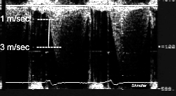
M-mode echocardiography and the Mathematica Program
Eric Sincoff, M.D.
Matlab is a matrix based computer language similar to Fortran or Basic but easier to implement and more powerful. Since digitized images are nothing more than matrices with each member of the matrix representing a pixel color or gray scale intensity, Matlab is well suited for this type of processing.
The image processing required to obtain velocity versus time data from a raw Doppler image provides an example of the power of Matlab in the processing of echocardiographic images.

The Matlab subroutines on this page should be downloaded as a set and can be used by anyone with access to Matlab version 3.0 or higher and the image processing toolbox. This can be better understood if one has a basic understanding of image processing which follows in the form of a small glossary.
Basic Glossary of Image Processing
It should be noted that this glossary is in pedagogical rather than alphabetical order.
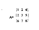
Matrix - A set of numbers as shown by [A]. [A] is a simple 3 by 3 matrix a typical image may be 200 by 200 or even greater. Each member of the matrix represents a pixel of the image and its value denotes a color or a gray scale value.

Fast Fourier Transform (FFT) - The method of representing a function as a series of sine and cosine functions. The Fourier transform can be applied in a discrete manner to a matrix and in so doing transforms the image from the spatial domain to the frequency domain. The image can then be processed in the frequency domain and then by use of the inverse fast Fourier transform the processed image can be brought back to the spatial domain. Matlab has built in functions for doing FFT and IFFT.
Convolution - An operation of linear algebra that allows one to filter an image in the spatial domain. It should be noted that convolution in the spatial domain is equal to multiplication in the frequency domain. For example,

[C] was obtained by placing [B] over each member of [A], multiplying the members of [A] by those of [B] that lie over them, adding up the resulting values of the multiplication, and letting the result of the addition be the corresponding member of [C]. For example [C](2,2)=1*1+2*2+3*2+1*3=14. In most image processing only the central part of the convolution is desired. So the central part of [C] is

Alternatively [C] could have been obtained by taking the FFT of [A] and [B] multiplying them and taking the IFFT of the result.
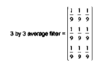
Linear Spatial Filtering - In the spatial domain a linear filter is just the central part of the convolution of a image matrix and a filter mask. Some examples of filter masks are as follows

The above filter takes the average of each pixel and its 8 neighbors and replaces the pixel with the result. This is done by taking 1/9 of each pixel value and adding up the results of the multiplication.
Another filter example is

This filter takes the difference of the pixels lying just above and below a pixel and can be used to detect changes in pixel intensity along an edge. The above are only two examples of different linear filters and the Matlab routines here make use of many more.
Non-Linear Filtering - Any filter that makes use of a non-linear process. For example, replacing each pixel with the median of its neighbors (remember that median is the middle value of a set whereas mean is the average value of a set). Another example would be to replace each pixel with the standard deviation of it neighbors. Many of the Matlab routines presented here make use of non-linear filtering.
Connectivity-The number of connected pixels. This can be a number from 0 to 8; if one allows all of the background to be equal to zero and not included in computing the connectivity. For example,

The above definitions and concepts form only a very simple primer in this highly developed field. Some books for further reference are Digital Image Processing by Gonzalez and Woods, Cardiac Imaging and Image Processing by Collins and Skorton.
another calling program-loads data,etc.
preprocesses the image-calls several different filters
a clustering filter-a non-linear filter
finds the connectivity of the image
calculates pressure gradient from Bernoulli equation
reconstructs the pressure plot
%This function postprocesses the t and v data
function [t,v]=postpro(t,v,tref,vref,tscale,vscale)
%Throw out garbage
for i=3:length(v)-2;
if v(i)
Back to E-chocardiography Home Page.
The contents and links on this page were last verified on December 24, 1998.
%This is a function to test the program with most of its features
function [t,v,delp,p,dpdt,dpdtmax,...
negdpdtmax,dpdtdivkp,vmax,vpm]=test

[t,v]=autvandt;
[delp]=deltap(t,v);
[p]=reconst(delp,t);
[dpdt,dpdtmax,negdpdtmax,dpdtdivkp,vmax,vpm]=cf(p,0,t);


clf;subplot(1,3,1);plot(t(1:length(p)),p,'r-');subplot(1,3,2);plo
t(p(1:length(dpdtdivkp)),dpdtdivkp,'g.')...
;subplot(1,3,3);plot(t(1:length(dpdt)),dpdt,'b+');
%This function automatically finds the edge of a BMP MR and
returns
%v and t it calls several other functions that actually do the
filtering and
%edge detection of the image

function [t,v]=autvandt

%Input the BMP file
check='n';
while check=='n',
 fname=input('The name of the MR V-profile file ','s')
 check=input('Are you sure this is the file-y or n ','s')
end;


%Enter time and velocity scales this allows the user to set a
certain number of pixels on the image
%to a known velocity and time period
tref=input('What is the time reference in ms? ')
vref=input('What is the velocity reference in m/s? ')

%Read in the file using the header info
[data,map]=bmpread(fname);

%Image the matrix data
clf;hold
on;colormenu;colormap(map);image(data);axis('equal');axis('ij');

%What type of scan
ttorte=input('Is this a trans-thoracic or trans-esophegeal?(enter
te or tt)  ','s')

%Get reference points for v and t scaling
goon='n';
while goon=='n';
 t1=0;t2=0;v1=0;v2=0;blank=0;

 [t1,blank]=ginput(1);
 hold on;plot(t1,blank,'r+');
 [t2,blank]=ginput(1);
 plot(t2,blank,'r+');
 [blank,v1]=ginput(1);
 plot(blank,v1,'g+');
 [blank,v2]=ginput(1);
 plot(blank,v2,'g+');
 goon=input('Are these the points you want? y or n ','s')
end;
tdist=abs(t1-t2)
vdist=abs(v1-v2)
tscale=tref/tdist;
vscale=vref/vdist;

%Crop the image to the area of interest (area of initial dp/dt)
goon='n';
while goon=='n';
 cropdata=0;
 cropdata=imcrop;clf,hold
on,image(cropdata);axis('equal');axis('ij')
 goon=input('Is this the area you want? y or n ','s')
end;

%Prefilter the data
%This calls another function preproc.m that does some of the
initial preprocessing of the image
[prefiltim,mask,xv,yv]=preproc(cropdata,map);
roiorwhole=menu('ROI or Whole Image','ROI','Whole')
if roiorwhole==1;
 prefiltim=prefiltim.*mask;
 rev=ones(size(cropdata))-mask;
end;


%Detect the edge from the filtered
%Gives the user the choice of 3 different edge detection
algorithims
%edgefin3,raster,or edgefin6.  These routines were found to be
most successful
%but are far from perfect.
clf,image(prefiltim),colormap(map),axis('equal'),axis('ij');
method=menu('Method','Column','Raster','Reverse Column','Modified
Column')
if method==1;
 [t,v]=edgefin3(prefiltim,map,tscale,vscale,ttorte);
elseif method==2;
 [t,v,cost]=raster(prefiltim,map,tscale,vscale,ttorte);
elseif method==3;
 [t,v]=edgefin6(prefiltim,map,tscale,vscale,ttorte);
elseif method==4;
 [t,v]=edgefin7(prefiltim,map,tscale,vscale,ttorte);
end;


%Scale and normalize the data (scales the values obtained from
the image
%to m/s and s
t=(t-t(1))*tscale;
v=(v-v(1))*vscale;
%Filters that enhance the image(some of them)
function [filtim,mask,xv,yv]=preproc(orig,map)

clf;subplot(2,1,1);colormenu;colormap(map);image(orig);axis('equa
l');axis('ij');

%Present the user with the various filter options
ch=0;roi=0;
while ch~=11
 ch=menu('Select the desired filter','Histogram Equalization',...
 'Unsharp Mask','Median Filter','Wiener Filter','Highpass
Butterworth',...
 'Contrast Enhance','Threshold','Cluster','Region of
Interest','Remove Isolated Pixels','End' )

 if roi==1;
  orig=orig.*mask;
 end;

 if ch==1
  %Compute the equalized histogram
  [orig]=eqhist(orig,map);
 elseif ch==2
  %Compute unsharp masked image
  a=input('What value for A (constant used in unsharp masking)?
')
  [orig]=unmask(a,orig);
 elseif ch==3
  %Perform a median filter operation
  [orig]=medfilt2(orig,[10,2]);
 elseif ch==4
  %Perform a Wiener filter
  [orig,noise]=wiener2(orig,[7,7]);
 elseif ch==5
  %Perform a HPBF with highfrequency enhance(doesn't work)
  [orig]=hpbf(orig);
 elseif ch==6
  %Perform contrast enhancing laplacian filter
  [orig]=cenhance(orig);
 elseif ch==7
  %Threshold the image
  [m,n]=size(orig);
  disp('Pick a point on the outside of the curve')
  [q,p]=ginput(1);
  th=mean2(orig(p-5:p+5,q-5:q+5))+std2(orig(p-5:p+5,q-5:q+5));
  for c=1:m;
   for r=1:n;
    if orig(c,r)>th;
     orig(c,r)=256;
   else;
    orig(c,r)=1;
   end;
  end;
 end;
 elseif ch==8
  %Cluster the image
  [orig]=cluster(orig);
 elseif ch==9
  %Region of interest
  roi=menu('Options','On','Off','Define')
  if roi==3;
   [mask,xv,yv]=roipoly;
   rev=ones(size(orig))-mask;
   reforig=orig;
   roi=1;
  elseif roi==2;
   orig=orig+(reforig.*rev);
  end;
 elseif ch==10
  [conn,sim,bw]=connect(orig,map);
  orig=orig.*bw;
  th=input('Input the highest connectivity of those pixels that
you wish to remove ')
  [m,n]=size(conn);
  mult=zeros(m,n);
  for r=1:m;
   for c=1:n;
    if conn(r,c)>=th;
    mult(r,c)=1;
    end;
   end;
  end;
  orig=orig.*mult;
 elseif ch==11;
  end;
if roi~=1;

subplot(2,1,2),colormap(map);image(orig);axis('equal');axis('ij')
;
elseif roi==1;
 hold
on,subplot(2,1,2),colormap(map);image(orig+(reforig.*rev));plot(x
v,yv,'r');axis('equal');axis('ij');
end;
end;
if roi==1|roi==2|roi==3;
 filtim=orig+(reforig.*rev);
else;
 filtim=orig;
end;
%Function to do unsharp masking
function [filtorig]=unmask(a,orig)

%Perform unsharp masking
%Compute the filtering matrix
w=9*a-1;
f=(-1/9).*ones(3,3);f(2,2)=w/9;
filtorig=filter2(f,orig);
%Contrast Enhancing Filter
%This is essentially a unsharp masking filter in the Matlab
%image processing library (see help fspecial in Matlab for
details)

function [cenhance]=cenhance(orig)

sh=input('What shape of filter do you want? ')

h=fspecial('unsharp',sh);
cenhanc=filter2(orig,h);
%A function to find the edge by placing the edge point of each
column where
%the change in pixel intensity is greatest for that column

%This function finds the edge of the filtered image

function [t,v]=edgefin3(im,map,tscale,vscale,ttorte)

disp('Enter the point of origin')
[tref,vref]=ginput(1);
disp('Enter the point of to stop')
[tstop,blank]=ginput(1);
disp('Enter velocity limit')
[blank,vstop]=ginput(1);
[m,n]=size(im);
vref=round(vref);
tref=round(tref);
vstop=round(vstop);
tstop=round(tstop);
gradient=diff(im,1);
if ttorte=='te';
 gradient=flipud(gradient);
 vref=m-vref;
 vstop=m-vstop;
end;
[sortgrad,index]=sort(abs(gradient(vref:vstop,:)));
t=tref:tstop;
[k,l]=size(index);
v=index(k,tref:tstop)+vref-1;

[t,v]=postpro(t,v,tref,vref,tscale,vscale);

%Display the results of the edge superimposed on the image
[m,n]=size(im);
if ttorte=='tt';
 clf,hold
on,colormap(map),image(im),plot(t,v,'r.'),axis('equal'),axis('ij'
);
end;
if ttorte=='te';
  clf,hold
on,colormap(map),image(im),plot(t,m-v,'r.'),axis('equal'),axis('i
j');
end;
pause;
%A function to find the edge using raster tracking
%This routine goes from pixel to pixel and compares the cost of
the path
%between a pixel and each of it neighbors that lie in the column
to the right of it
%the next pixel is the one with the lowest cost(works fair)


function [t,v,cost]=raster(im,map,tscale,vscale,ttorte)

clf,colormap(map),image(im),colormenu,axis('ij'),axis('equal');

disp('Enter the point of origin')
[tref,vref]=ginput(1);
disp('Enter the point of to stop')
[tstop,blank]=ginput(1);
disp('Enter velocity limit')
[blank,vstop]=ginput(1);
[m,n]=size(im);
vref=round(vref);
tref=round(tref);
vstop=round(vstop);
tstop=round(tstop);

t=[tref:tstop];
v(1)=vref;

if ttorte=='te';
 im=flipud(im);
 vref=m-vref;
 vstop=m-vstop;
end;

%Determine the cost matrix of the image in the vertical
direction,note cost as defined here is really the inverse of cost
g1=diff(im);
g2=diff(diff(im));
cost=g1(1:m-2,:)+g2(1:m-2,:);

%Define the search path starting at tref,vref and going to tstop
and max of vstop
%Search east for 1 pixel and s or n for 10 pixels
n=2;
rev=0;
dir=1;
while n<=length(t);
 cost1=cost(v(n-1),t(n-1));
 if rev==1;
  dir=dir*(-1);
 end;
 if v(n-1)>=vstop;
  dir=-1;
 end;
 if v(n-1)<=vref & n>2;
  dir=1;
 end;

 if vstop-v(n-1)<=10 & dir==1;
  limit=vstop-v(n-1);
 elseif v(n-1)-vref<=10 & n>length(t)/2 & dir==-1;
  limit=v(n-1)-vref;
 else;
  limit=9;
 end;

 for ind=0:limit;
  indpost=ind*dir;
  deltacost(ind+1)=abs(cost1-cost(v(n-1)+indpost,t(n)));
 end;
 [deltacost,index]=sort(deltacost);
 if dir==-1;
  index=-1*index;
 end;
 v(n)=v(n-1)+index(1)+1;
 %If 5 or more succsessive v are similar or vstop is reached then
reverse direction
 rev=0;
 if n>6;
  if
v(n)>=mean(v(n-5:n-1))-.5*std(v(n-5:n-1))&v(n)<=mean(v(n-5:n-1))+
.5*std(v(n-5:n-1));
   rev=1;
  end;
 end;
 n=n+1;
end;
if ttorte=='tt';
 clf,hold
on,colormap(map),image(im),plot(t,v,'r.'),axis('equal'),axis('ij'
);
end;
if ttorte=='te';
  clf,hold
on,colormap(map),image(flipud(im)),plot(t,m-v,'r.'),axis('equal')
,axis('ij');
end;
pause;
%A function to find the edge(modified from edgefin3.m)
%This function finds the edge of the filtered image by placing
the edge point for each column where
%the pixel intensity is outside the range of the mean +or- the
std of the
%3 pixels ahead of it processing goes from the velocity to to the
zero velocity
function [t,v]=edgefin6(im,map,tscale,vscale,ttorte)
disp('Enter the point of origin')
[tref,vref]=ginput(1);
disp('Enter the point of to stop')
[tstop,blank]=ginput(1);
disp('Enter velocity limit')
[blank,vstop]=ginput(1);
[m,n]=size(im);
vref=round(vref);
tref=round(tref);
vstop=round(vstop);
tstop=round(tstop);
t=[tref:tstop];
for c=tref:tstop;
col=im(vref:vstop+10,c);
found=0;
r=vstop;
while found==0 & r>vref;
bigchange1=mean(col(r+2-vref:r+5-vref))+(1.*std(col(r+2-vref:r+5-
vref)));
bigchange2=mean(col(r+2-vref:r+5-vref))-(1.*std(col(r+2-vref:r+5-
vref)));
if col(r-vref+1)>bigchange1 | col(r-vref+1)
%A function to find the edge(modified from edgefin6.m)
%This function finds the edge of the filtered image by placing
the edge point for each column where
%the difference in pixel intensity between two column pixels
meets a certain limit
function [t,v]=edgefin7(im,map,tscale,vscale,ttorte)
disp('Enter the point of origin')
[tref,vref]=ginput(1);
disp('Enter the point of to stop')
[tstop,blank]=ginput(1);
disp('Enter velocity limit')
[blank,vstop]=ginput(1);
[m,n]=size(im);
vref=round(vref);
tref=round(tref);
vstop=round(vstop);
tstop=round(tstop);
t=[tref:tstop];
for c=tref:tstop;
col=im(vref:vstop+10,c);
grad=abs(diff(col));
maxgrad=max(grad);
mingrad=min(grad);
lim=.5.*(maxgrad);
for r=1:length(grad);
if grad(r)>=lim;
v(c-tref+1)=vref+r+1;
end;
end;
end;
[t,v]=postpro(t,v,tref,vref,tscale,vscale);
%Display the results of the edge superimposed on the image
[m,n]=size(im);
if ttorte=='tt';
clf,hold
on,colormap(map),colormenu,image(im),plot(t,v,'r.'),axis('equal')
,axis('ij');
end;
if ttorte=='te';
clf,hold
on,colormap(map),image(im),plot(t,m-v,'r.'),axis('equal'),axis('i
j');
end;
pause;
%This function clusters the image into subsets
%Clustering is defined here as taking an image and finding the
average pixel value
%and standard deviation of two user defined regions in the image
and then examining
%each pixel in the image to see if it lies in the range of the
average +or- the std
%of each region and placing that pixel in either c1 if it lies in
the range of region 1
%or c2 if in the range of region2 or c3 if not in either range
function [orig,c1,c2,c3]=cluster(orig,map)
[m,n]=size(orig);
c1=zeros(m,n);
c2=zeros(m,n);
c3=zeros(m,n);
colormap(map),colormenu,image(orig),axis('equal'),axis('ij');
region1=imcrop;
region2=imcrop;
avg1=mean2(region1);
avg2=mean2(region2);
sd1=std2(region1);
sd2=std2(region2);
for r=1:m;
for c=1:n;
if orig(r,c)>(avg1-(1*sd1)) & orig(r,c)<(avg1+(1*sd1));
c1(r,c)=orig(r,c);
elseif orig(r,c)>(avg2-(1*sd2)) & orig(r,c)<(avg2+(1*sd2));
c2(r,c)=orig(r,c);
else;
c3(r,c)=orig(r,c);
end;
end;
end;
%This function examines the connectivity of each image pixel
% Similarity is defined as the absolute value of the difference
of each pixel and its
%connected neighbors
%conn=matrix of the connectivity of each pixel,sim=matrix of
similarity of each pixel,bw=binary image
function [conn,sim,bw]=connect(orig,map)
maxpix=max(max(orig));
minpix=min(min(orig));
connectivity=0;
similarity=0;
%Changes the image to a binary setting the background(lowest
pixel value) to
%zero and all others to 1
bw=im2bw(orig./maxpix,(minpix/maxpix)+eps);
[m,n]=size(bw);
conn=zeros(m,n);
sim=zeros(m,n);
%Go through image pixel by pixel and calculate the connectivity
and similarity of each
for r=2:m-1;
for c=2:n-1;
if bw(r,c)==1;
for k=-1:1;
if bw(r+k,c-1)==1;
connectivity=connectivity+1;
similarity=similarity+abs(orig(r,c)-orig(r+k,c-1));
end;
if bw(r+k,c+1)==1;
connectivity=connectivity+1;
similarity=similarity+abs(orig(r,c)-orig(r+k,c-1));
end;
end;
if bw(r+1,c)==1;
connectivity=connectivity+1;
similarity=similarity+abs(orig(r,c)-orig(r+1,c));
end;
if bw(r-1,c)==1;
connectivity=connectivity+1;
similarity=similarity+abs(orig(r,c)-orig(r-1,c));
end;
conn(r,c)=connectivity;
sim(r,c)=similarity;
connectivity=0;
similarity=0;
end;
end;
end;
%This function computes and plots the delta P vs. time using data
%from autvandt using the modified Bernoulli equation
function [deltap]=deltap(t,v)
deltap=4.*(v.^2);
clf,hold on,plot(t,deltap),title('Delta P Across Mitral Valve
Versus Time'),...
xlabel('time(ms)'),ylabel('Delta P (mmHg)');
%Function to Reconstruct P wave from delta P and systolic BP(only
an approximation of the true P wave)
%In theory one could use a Swan-Ganz wedge pressure to get the
pressure in the left atrium and use that as
%a baseline pressure and add the pressure gradient to the
baseline giving a true pressure wave (if done in real time)
function [p]=reconst(delp,t)
%Get the max systolic BP
sysbp=input('What is the max systolic BP ')
%The time of max systolic BP is when dP/dt =0
%Find the index of max systolic BP
[dp,d,dt]=dpdtdvdt(delp,t,t);
dpdt=dp./dt;
ilowabsdpdt=0;
i=0;
while ilowabsdpdt==0;
i=i+1;
if dpdt(i)>0 & dpdt(i+1)<0;
ilowabsdpdt=i;
end
end
%Find the delta P at max systolic BP
deltapilow=(delp(ilowabsdpdt)+delp(ilowabsdpdt+1))/2;
%Get the constant of integration
c=sysbp-deltapilow;
%Solve for P
p=delp+c;
%This Function Calculates Many of The Parameters in the Book
Cardiac Catheterization by Grossman Ch. 20
function [dpdt,dpdtmax,negdpdtmax,dpdtdivkp,vmax,vpm]=cf(p,v,t)
%Note p=pressure,v=volume,t=time; volume is not used in any of
these calculations
%dpdt=dp/dt
%Get dp dv and dt
%Calls a routine that simply calculates dp,dv,dt
%Note t is sent for v so the routine does not crash but is not
used in the calculation
%so dv=dt in this function call, dv is not used in any
calculations
[dp,dv,dt]=dpdtdvdt(p,t,t);
%Get end diastolic pressure by assuming it is the lowest pressure
%of the cardiac cycle
edp=min(p);
%Use DP or TP
%These are defined in Grossman TP=total pressure (measured
pressure)
%DP=TP-edp
dportp=input('Type dp=1 or tp=2 for what you want used in these
calculations')
%P is measured as TP so transform P into DP if user wants DP
if dportp==1;
p=p-edp;
end;
%Calculate dp/dt and max dp/dt and max(-dp/dt)
%Note that in Matlab ./ and .* are not the same as their linear
algebra counterparts
%but simply dividing or multiplying each member by its
corresponding member
dpdt=dp./dt;
%Find dp/dtmax and min for the set of data
dpdtmax=max(dpdt);
negdpdtmax=min(dpdt);
%Find Vmax see method on page 251 of Grossman
k=input('What value of K do you want(normally between 28 and 32)
')
for i=1:length(dpdt);
dpdtdivp(i)=dpdt(i)./((p(i)+p(i+1))/2);
end;
dpdtdivp=dpdtdivp';
dpdtdivkp=dpdtdivp./k;
for i=1:length(dpdt);
if dpdt(i)==max(dpdt);
imaxdpdt=i;
end
end
for i=1:length(dpdtdivp);
if dpdtdivp(i)==max(dpdtdivp);
imaxdpdtdivp=i;
end
end
%This polynomial fitting to get Vmax has been comented out as it
sometimes crashes
%It can be uncommented by removing the % before each line
%if imaxdpdtdivp~=imaxdpdt;
%[pol]=polyfit(p(imaxdpdtdivp:imaxdpdt),...
%dpdtdivp(imaxdpdtdivp:imaxdpdt),4);
%vmax=polyval(pol,0);
%else;
vmax=dpdtdivkp(imaxdpdt);
%end;
% Get TP back from DP if transformed
if dportp==1;
tp=p+edp;
else tp=p;
end;
%Calculate Vpm
dpdtdivtp=(dp./dt)./(p(1:length(dpdt)));
vpm=max(dpdtdivtp);
%This function calculates dp, dv dt from a matrix of data;
function [dp,dv,dt]=dpdtdvdt(p,v,t);
if size(p)~=size(v); elseif size(p)~=size(t); elseif
size(v)~=size(t);
n=1;
else;
n=0;
end;
if n==1;
disp('Matrices must be same size')
end;
if n==0;
[dt]=diff(t);
[dp]=diff(p);
[dv]=diff(v);
end;
%This function does histogram equalization a set number of times
function [eqorig]=eqhist(orig,cmap)
%Compute the equalized histogram
[i,j]=size(orig);
eqorig=orig;
%Compute the initial histogram of the image
[n,y]=imhist(eqorig,cmap);
%Compute the new equalized histogram
c(1)=n(1);
for q=2:length(n);
c(q)=c(q-1)+n(q);
end;
tot=i*j;
t=(c./(tot));
%Calculate the histogram equalized image
[eqorig]=(histeq(orig./256,t)).*256;